1、这个函数表现为S形曲线:
Plot[5*f, {x, -5, 5}, AspectRatio -> Automatic]

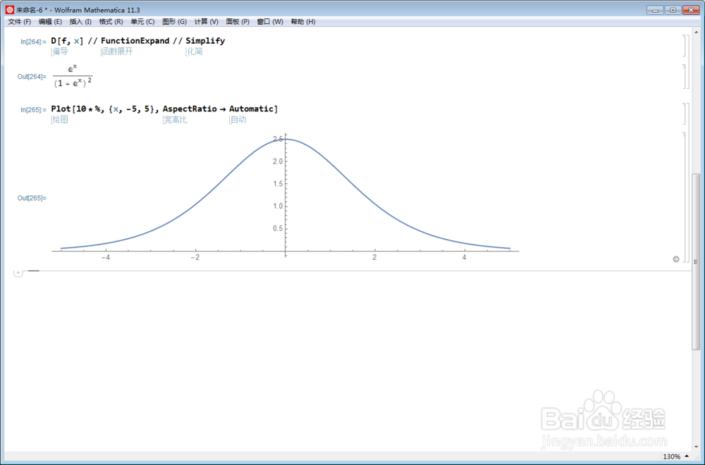
2、它是单调递增函数:
In[0]:= D[f, x] // FunctionExpand // Simplify
Out[0]= E^x/(1 + E^x)^2
3、它的值域是[0,1],以y=0和y=1为渐近线:
In[0]:= Limit[f, x -> -Infinity]
Out[0]= 0
In[0]:= Limit[f, x -> +Infinity]
Out[0]= 1

4、它是中心对称图形,左侧是下凹曲线,右侧是上凸曲线:
In[0]:= D[f, {x, 2}] // FunctionExpand // Simplify
Out[0]= -((E^x (-1 + E^x))/(1 + E^x)^3)

5、它可以把所有数据归拢到0和1之间,且不同的数据,仍旧不同:
In[0]:= data = RandomReal[10, 10]
Out[0]= {0.143454, 4.77656, 1.28397, 0.799853, 4.48448, 9.89067,
9.6725, 7.84665, 2.66615, 7.23431}
In[0]:= LogisticSigmoid[#] & /@ data
Out[0]= {0.535802, 0.991645, 0.783125, 0.689943, 0.988843,
0.999949, 0.999937, 0.999609, 0.935, 0.999279}

6、与此功能类似的函数,可以是ArcTan[x]:

7、对比一下这两个函数的图像:
Plot[{2*ArcTan[x]/Pi + 1, 2 f}, {x, -2, 2}, AspectRatio -> Automatic]
