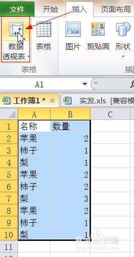
1、选定数据区域A1:B10,插入>>>数据透视表,如下图
Select the data area A1:B10, insert the >>> PivotTable, as shown below
2、表/区域中自动输入了单元格地址,如果有误,可直接修改,根据需要选择放置数据透视表位置,本例以新工作表为例,单击“确定”按钮,如下图
The cell address is automatically entered in the table/area. If there is an error, you can directly modify it. Select the position of the PivotTable as needed. In this example, take the new worksheet as an example and click the “OK” button, as shown below.

3、把“名称”拉到“行标签”,“数量”拉到“数值”区域,透视表将自动计算结果,如下图
Pull the "name" to the "row label", the "quantity" to the "value" area, the pivot table will automatically calculate the result, as shown below

1、选定要放置计算结果的首个单元格,如D1,数据>>>合并计算
Select the first cell to place the calculation result, such as D1, data >>> merge calculation
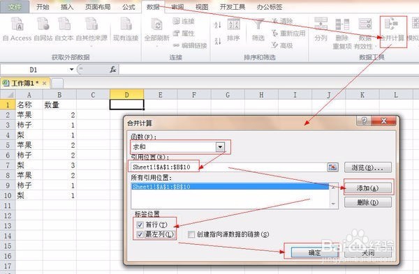
2、“函数”选择“求和”,鼠标放在“引用位置”框中,再选择数据区域A1:B10,框中将自动输入引用位置的单元格地址,单击“添加”按钮,再勾选“首行”和“最左列”复选框,最后单击“确定”按钮,如下图
"Function" select "summation", mouse in the "reference position" box, and then select the data area A1:B10, the box will automatically enter the cell address of the reference location, click the "Add" button, and then check " The first line and the leftmost column check box, and finally click the "OK" button, as shown below
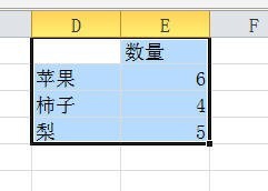
3、结果如下图,Excel已自动汇总了数据,并对数量求和,在D1单元格输入名称就可以了。
The result is as shown below. Excel has automatically summarized the data and summed the quantities. Enter the name in the D1 cell.