1、GraphPlot[{1 -> 2, 1 -> 3, 2 -> 3, 1 -> 4, 2 -> 4, 1 -> 5}]
绘制一个图(Graph)。

2、LayeredGraphPlot[{1 -> 2, 1 -> 3, 2 -> 3, 1 -> 4, 2 -> 4, 1 -> 5}]
生成图(Graph)的分层图。

3、TreePlot[{1 -> 4, 1 -> 6, 1 -> 8, 2 -> 6, 3 -> 8, 4 -> 5, 7 -> 8}]
生成树状图。
即使不是一颗“树形图”,也可能运行:
TreePlot[{1 -> 2, 1 -> 3, 2 -> 3, 1 -> 4, 2 -> 4, 1 -> 5}]


4、LineIntegralConvolutionPlot生成一个矢量图的线性积分卷积图:
LineIntegralConvolutionPlot[{Sin[2 x], Cos[3 y]}, {x, -1, 1}, {y, -0.6, 0.6}]
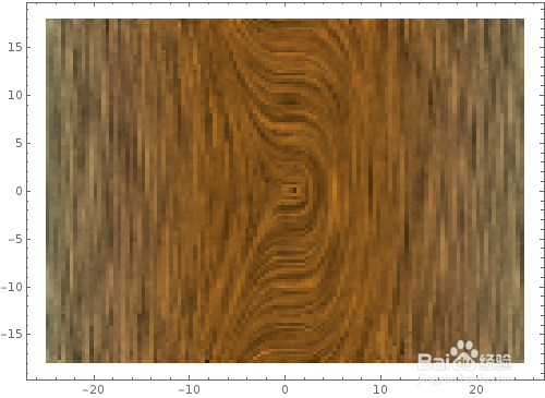
把这个效果作用于图片:
LineIntegralConvolutionPlot[{{Sin[2 x], Cos[3 y]},图片}, {x, 0, 500}, {y,0, 376}]


5、ListCurvePathPlot,用光滑曲线连接二维点列:
data = Table[{Cos[t], Sin[t]}, {t, RandomReal[{0, 2 Pi}, 50]}];ListPlot[data, AspectRatio -> Automatic]


6、data = Table[{{x, y}, {y, x - x^2}}, {x, -25, 25, 0.2}, {y, -18, 18, 0.2}];
ListLineIntegralConvolutionPlot[data]
绘制一个插值后的向量域的积分卷积图形。
ListStreamDensityPlot[data]
用插值的方法绘制流线图。
ListVectorDensityPlot[data]
用插值的方法绘制向量图。


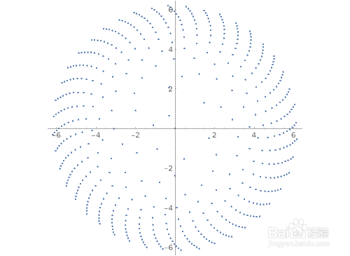
7、以等角间隔绘制一组数据(注意,数据为极半径):
ListPolarPlot[Table[{n, Log[n]}, {n, 500}]]
ListPolarPlot[Table[{n, Log[n]}, {n, 5000}]]
ListPolarPlot[Table[{n, Log[n]}, {n, 500}],Joined->True]


8、NicholsPlot绘制系统对应的Nichols图:
NicholsPlot[TransferFunctionModel[{{{10}}, (s (2 + s)) (4 + s)}, s],
ColorFunction -> Function[{x, y, f}, Hue[f]]]
NyquistPlot绘制系统对应的Nyquist图:
NyquistPlot[ TransferFunctionModel[{{{(10 (1 + 3 s)) (1 + 4 s)}},
(((1 + s) ( 2 + s)) (5 + s)) (6 + s)}, s]]


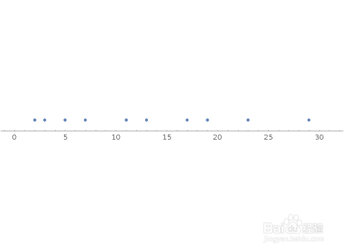
9、NumberLinePlot[Prime[Range[10]]]
NumberLinePlot[Prime[Range[100]]]
在数轴上标出数值对应的点。
NumberLinePlot[{Range[36], 2 Range[18],
3 Range[12], 4 Range[9], 6 Range[6]}]


10、ProbabilityPlot给出与数据相对应的正态分布的概率图:
Table[ProbabilityPlot[Range[0, 1, 0.025]^2, Joined -> True,
ColorFunction -> Function[{x, y}, f], PlotLabel -> f, PlotStyle -> Thick], {f, {Hue[x], Hue[y]}}]
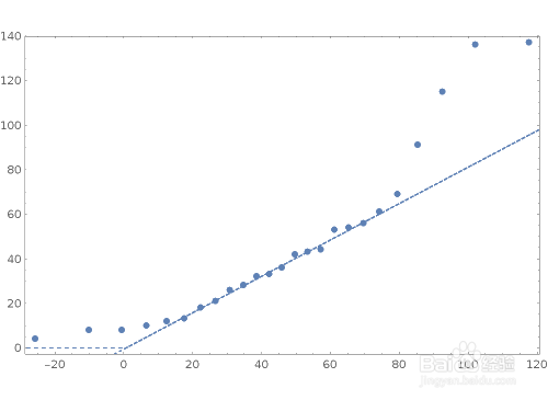
ProbabilityScalePlot给出与数据相对应的正态分布的概率图,并按照指定的规则进行缩放:
shuju = {8, 44, 91, 32, 4, 33, 8, 115, 61, 136, 18, 54, 43, 28, 56, 36, 137, 26, 53, 21, 69, 12, 13, 42, 10};ProbabilityScalePlot[shuju, "LogNormal", GridLines -> Automatic, GridLinesStyle -> "Classic", ImageSize -> {500,365}]
将数据与一个正态分布进行比较:
QuantilePlot[shuju]


11、根据等高线数据绘制地形图:
ReliefPlot[ Table[ y^2 + 6 Sin[x^2 + y^2]-x Sin[x+ y^2],
{x, -10.95, 10.95, 0.05}, {y, -15, 15, 0.05}],
ColorFunction ->Hue]


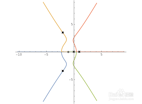
12、RootLocusPlot生成一个系统的根轨迹图:
RootLocusPlot[TransferFunctionModel[{{{k (1 + s)}},
((-1 + s) s) ( 16 + 4 s + s^2)}, s], {k, -1000,1000}]
13、RulePlot按照某种规则
RulePlot[CellularAutomaton[30], {{1}, 0}, 10]
RulePlot[CellularAutomaton[30], {{1}, 0}, 100]
用某个元胞自动机(rule30)的基本图形和规则构造图片。


14、TimelinePlot绘制时间轴线:
TimelinePlot[{Ctrl+world war1,Ctrl+world war2}]
绘制两次世界大战的时间轴。
